Adam Scott, MS, CSCS
“The standard for success of a foot march is very simple to measure: did the unit arrive at the destination at the prescribed time with the Marines in condition and required equipment present to accomplish the mission?”
– US Marine Corps Reference Publication (MCRP) 3-02A
The MCRP continues: “The success of the march will depend largely upon the thoroughness with which it is planned” (1). One of the key components of this process is estimating how long the march will take. Over flat, paved terrain the planning process is relatively simple. All we need is one simple equation:
EQUATION 1:
Time (t) equals Distance (d) divided by Speed (s):

Under such conditions, the US Army’s Field Manual for Foot Marches (FM 21-18) offers roughly the same recommendations as the USMC’s MCRP 3-02A: 4km/hr for daytime movement and 3.2 km/hr for nighttime movements (1,2). In the civilian world, speed recommendations are fairly similar – they typically range from 3-5 km/hr (4,5,9,13-15).
While these numbers represent an excellent starting point for planning movements, they don’t represent the realities that most mountain and tactical professional face. In the real world, there are a number of variables which will affect an individual’s (or unit’s) ability to move over ground. TABLE 1 contains seven (7) such variables (1-15).
TABLE 1: Seven (7) Factors Effecting Speed (1-15)

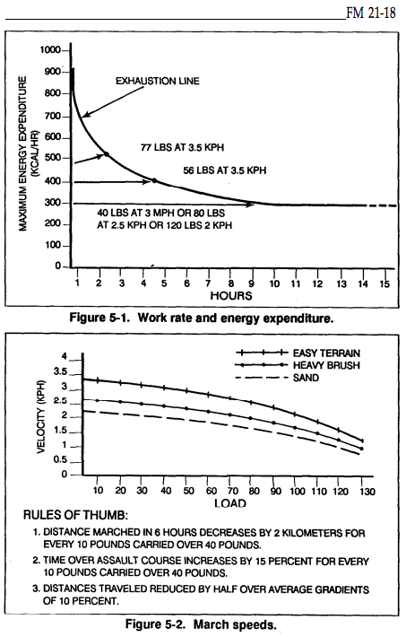
Military manuals take a rather simplistic approach to these seven variables. Basically, they are lumped into what FM 21-18 and MCRP 3-02A call “Cross-Country” travel. For military units, Cross-Country planning speeds drop to 2.5-2.6 km/hr for daytime travel and 1.6 km/hr for nighttime travel (1,2). * Note: FM 21-18 does include adjustments for loads over 40lbs, which will be addressed later.
Mountain professionals have taken a much more thorough approach to addressing these compounding factors. The Naismith Rule, originally published in 1892 by Scottish mountaineer, William Naismith, provides a “general rule of thumb” which establishes the relationship of horizontal to vertical movement (4,8,9).
Naismith’s rule has undergone many updates the last 100+ years, including: Tranter’s Correction, Aitken’s Correction (1977) and Langmuir’s Correction (1984) (4,8,9,14-15).
In addition to these “rules of thumb” there are also equations like Tobler’s Hiking Function and a model used by the Swedish military. Recently, new estimation tools have been developed which use power outputs and energetics (14-15) to estimate speeds.
Despite their differences, all of these rules and equations have one thing in common: they are trying to account for the variables mentioned above (TABLE 1). Research comparing the different methods has shown that they produce relatively similar predictions with decent accuracy (+/- 19-21%) (14).
A QUICK LOOK AT THE CURRENT “RULES” FOR ESTIMATING TRAVEL TIME (Warning, don’t get too caught up in the equations):
Naismith’s original rule was pretty simple, it consisted of two parts:
-
-
- Allow 1 hour for every 5 kilometers of travel.
- Add 1 hour for every 600m (2000ft) of ascent.
-
Based on his research in 1977, Aitken recommended the speed be dropped to 4km/hr. Then in 1984 Langmuir added two additional rules, bringing the total to 4.
-
-
- Allow 1 hour for every 4 kilometers of travel (Updated).
- Add 1 hour for every 600m (2000ft) of ascent (No change).
- Subtract 10 minutes for every 300m of gentle descent (5-12 degrees) (New).
- Add 10 minutes for every 300m of steep descent (>12 degrees) (New).
-
A quick calculation based on these rules reveals a horizontal to vertical relationship of approximately 7.93 to 1. So, according to the rule, 800m of horizontal travel should take roughly the same amount of time as 100m of vertical travel. In the research, this is often referred to as the “Efficiency Factor” (EF).
Granted, the true ratio varies from athlete to athlete, but Naismith’s early estimation turns out to be a relatively accurate generalization. An analysis of hill running records reveals ratios of 8 to 1 for men and 10 to 1 for women (13). Even cycling data suggests a similar relationship between horizontal and vertical movement: 8.2 to 1 (13).
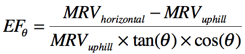
In our lab, our early tests have produced EF’s of between 4.8-9.9 to 1. So far our average is 7.3 to 1. We have also found that our athletes’ efficiency (i.e. EF) varies greatly depending on the slope of the incline (but more on that later). GRAPH 1 shows the average calculated EF from our first data collection. The EF equation we used is as follows:
EQUATION 2:
GRAPH 1: Measured Efficiency Factor (EF)

In 2013 the Geographic Resources Analysis Support System (GRASS) GIS project produced an equation based on Naismith’s Rule. The equation qualifies (1) uphill, (2) moderate downhill and (3) steep downhill effects.
EQUATION 3:
![]()
T = Travel Time (s)
△S = Horizontal Distance Traveled
△H = Vertical Distance Traveled
Moderate Downhill = -5 to -12 Degrees
Steep Downhill = >-12 Degrees
The final tool we want to introduce is Tobler’s Hiking Function. It is a mathematical equation which predicts human walking speeds based on slope. It was based on data collected from Swiss professor and cartographer, Eduard Imhof, in 1950.
Tobler’s equation shows that slope has an exponential relationship with speed. This relationship is similar to the results we have seen with our own lab rats.
EQUATION 4:
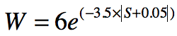
W = walking velocity (km/hr)
S = slope of the terrain (dh/dx)
OUR GOAL
Hopefully, you aren’t getting too bogged down in the calculations – that’s our job.
Over the next few weeks, we will be using these equations, research, and our own mini-experiments to develop a simple tool that military operators and mountain professionals can use to easily estimate their movement times. This process is going to encompass a few different parts:
First, there is the review of previous research. We are roughly 3 weeks into this process and are currently working to synthesize the information into a single source (you suffered through a little of that in the above article).
Second, we want to test a few of the currently available solutions which military and mountain athletes use to estimate their travel.
And, third, we will be revisiting our previously reported Five Rules For Rucking – to see if we can confirm or refute the rules.
In the end, tools like the one we hope to create (and those like it) offer a huge advantage in planning accuracy, and thus, mission success. Similar models are currently being used in everything from archeology, to search and rescue, to recreation, to professional safety (14).
* NOTE 1: US ARMY FM 21-18: Speed and Calorie Adjustments Based on Load
REFERENCES:
- (1) United States Marine Corps, Marine Corps Combat Development Command. Marine Corps Reference Publication 3-02A. Quantico, VA, JUNE 2004. http://www.trngcmd.marines.mil/Units/Northeast/TheBasicSchool/Academics/MarineForceReferencePublicationsMarineCorps.aspx. Accessed: 15 FEB, 2016.
- (2) Headquarters Department of the Army. U.S. Army Field Manual 18-21. Washington, DC, 01 JUNE 1990. http://armypubs.army.mil/doctrine/DR_pubs/dr_a/pdf/fm21_18.pdf. Accessed: NOV 18, 2015.
- (3) Sprott, J. Energetics of Walking and Running. sprott.physics.wisc.edu/technote/walkrun.html. Accessed: 10 FEB, 2016.
- (4) Langmuir, E. Mountaincraft and Leadership. Official Handbook of the Mountain Leader Training Boards of Great Britain and Northern Ireland. Edinburgh Scotland: Britain & Scottish Sports Council. 1984.
- (5) Reid, D and Falkenstein, C. Rock Climbs of Tuolumne Meadows (3rd ed.). Evergreen, Colorado, USA: Chockstone Press. p. 129. 1992.
- (6) Long, L and Srinivasan, M. Walking, running and resting under time distance and average speed constraints: optimality of walk – run – rest mixtures. J of Royal Soc; (10), 2014.
- (7) Hoogkamer, W, Taboga, P and Kram, R. Applying the cost of generating force hypothesis to uphill running. PeerJ; 2e(482). 2014.
- (8) Magyari-Saska, Z and Dombay, S. Determining minimum hiking time using DEM. Geographic Napocensis Annual VI, Nr(2). 2012.
- (9) Lauenstein, S, Wehrlin, J and Marti, B. Differences in horizontal vs. uphill running performance in male and female swiss world-class orienteers. J of Strn Cond Res; 27(11): 2952-2958. 2013.
- (10) Wayman, E. Energy efficiency doesn’t explain human walking? A new study of mammal locomotion challenges the claim that hominids evolved two-legged walking because of its energy savings. smithsonian.com. Published: 17 SEP, 2012. Accessed: 12 FEB 2016.
- (11) Paavolainen, L, Nummela, A and Rusko. Muscle power factors and VO2max as determinants of horizontal and uphill running performance. Scan J Med Sci Sports (10): 286-291. 2000.
- (12) Minetti, A, Moia, C, Fio, G, Susta, D and Ferretti, G. Energy cost of walking and running at extreme uphill and downhill slopes. J Appl Physiol; 93: 1039-1046. 2002.
- (13) Scarf, P. Route choice in mountain navigation Naismith’s rule and the equivalence of distance and climb. J of Sport Sci; 25(6): 719-726. 2007.
- (14) Iretenkauf, E. Analyzing Tobler’s hiking function and Naismith’s rule using crowd-sourced GPS data. Pennsylvania State University. Published: 30 OCT, 2013. https://gis.e-education.psu.edu/…/Irtenkauf… Accessed: 13 FEB 2016.
- (15) Leuthausser, U. About walking uphill: time required, energy consumption and the zigzag transition (English Version 1). Published: 21 FEB 2013. www.sigmdewe.com. Leuthausser Sustemanalysen. Accessed 13 FEB 2016.